如何在 PyTorch 中使用 skip-gram 结构实现 Word2Vec算法。将学习自然语言处理中用到的词嵌入概念。词嵌入对于机器翻译来说很有用。
词嵌入
在处理文本中的字词时,需要分析数千个字词类别;词汇表中的每个字词对应一个类别。对这些字词进行独热编码效率很低,因为独热向量中的大多数值将为 0。如果对独热输入向量与第一个隐藏层进行矩阵乘法运算,结果将生成一个有多个值为 0 的隐藏输出向量。为了解决这个问题并提高网络的效率,将使用嵌入功能。嵌入其实就是全连接层,和你之前看过的层级一样。将此层级称为嵌入层,将权重称为嵌入权重。将跳过与嵌入层的乘法运算步骤,直接从权重矩阵里获取隐藏层的值。这是因为独热向量与矩阵相乘后,结果是“开启”输入单元的索引对应的矩阵行。
Word2Vec
Word2Vec 算法通过查找表示字词的向量,得出更高效的表示法。这些向量也包含关于字词的语义信息。出现在相似上下文里的字词将具有相互靠近的向量,例如“coffee”、“tea”和“water”。不同字词的向量相互之间离得更远,在向量空间里的距离可以表示字词之间的关系。将使用 skip-gram 结构和负采样,因为 skip-gram 的效果比 CBOW 好,并且负采样的训练速度更快。对于 skip-gram 结构,传入一个字词,并尝试预测它在文本里的上下文字词。这样便能训练网络学习出现在相似上下文里的字词的表示法。
加载数据
加载数据并将其放入 data 目录中。
# read in the extracted text file with open('data/text8/text8') as f: text = f.read() # print out the first 100 characters print(text[:100]) 预处理
预处理文本,使训练流程更方便。utils.py 文件中的 preprocess 函数将执行以下几个操作:
- 将所有标点转换为标记,因此“.”变成
<PERIOD>。虽然此数据集没有任何标点,但是这一步对其他 NLP 问题来说很有用。 - 删除在数据集中出现次数不超过 5 次的字词。这样能够显著减少数据噪点带来的问题,并且能够改善向量表示法的质量。
- 返回由文本中的一些字词构成的列表。
utils.py
import re from collections import Counter def preprocess(text): # Replace punctuation with tokens so we can use them in our model text = text.lower() text = text.replace('.', ' <PERIOD> ') text = text.replace(',', ' <COMMA> ') text = text.replace('"', ' <QUOTATION_MARK> ') text = text.replace(';', ' <SEMICOLON> ') text = text.replace('!', ' <EXCLAMATION_MARK> ') text = text.replace('?', ' <QUESTION_MARK> ') text = text.replace('(', ' <LEFT_PAREN> ') text = text.replace(')', ' <RIGHT_PAREN> ') text = text.replace('--', ' <HYPHENS> ') text = text.replace('?', ' <QUESTION_MARK> ') # text = text.replace('\n', ' <NEW_LINE> ') text = text.replace(':', ' <COLON> ') words = text.split() # Remove all words with 5 or fewer occurences word_counts = Counter(words) trimmed_words = [word for word in words if word_counts[word] > 5] return trimmed_words def create_lookup_tables(words): """ Create lookup tables for vocabulary :param words: Input list of words :return: Two dictionaries, vocab_to_int, int_to_vocab """ word_counts = Counter(words) # sorting the words from most to least frequent in text occurrence sorted_vocab = sorted(word_counts, key=word_counts.get, reverse=True) # create int_to_vocab dictionaries int_to_vocab = {ii: word for ii, word in enumerate(sorted_vocab)} vocab_to_int = {word: ii for ii, word in int_to_vocab.items()} return vocab_to_int, int_to_vocab import utils # get list of words words = utils.preprocess(text) print(words[:30]) # print some stats about this word data print("Total words in text: {}".format(len(words))) print("Unique words: {}".format(len(set(words)))) # `set` removes any duplicate words 字典
将创建两个字典,一个将字词转换为整数,另一个将整数转换为字词。同样在 utils.py 文件里使用一个函数完成这个步骤。create_lookup_tables 的输入参数是一个文本字词列表,并返回两个字典。
- 按照频率降序分配整数,最常见的字词“the”对应的整数是 0,第二常见的字词是 1,以此类推。
创建好字典后,将字词转换为整数并存储在 int_words 列表中。
vocab_to_int, int_to_vocab = utils.create_lookup_tables(words) int_words = [vocab_to_int[word] for word in words] print(int_words[:30]) 二次采样
“the”、“of”和“for”等经常出现的字词并不能为附近的字词提供很多上下文信息。如果丢弃某些常见字词,则能消除数据中的一些噪点,并提高训练速度和改善表示法的质量。Mikolov 将这个流程称为二次采样。对于训练集中的每个字词 𝑤𝑖,将根据某个概率丢弃该字词,公式为:

其中 𝑡t 是阈值参数,𝑓(𝑤𝑖) 是字词 𝑤𝑖在总数据集中的频率。
对 int_words 中的字词进行二次采样。即访问 int_words 并根据上面所示的概率 𝑃(𝑤𝑖) 丢弃每个字词。注意,𝑃(𝑤𝑖)表示丢弃某个字词的概率。将二次采样的数据赋值给 train_words。
from collections import Counter import random import numpy as np threshold = 1e-5 word_counts = Counter(int_words) #print(list(word_counts.items())[0]) # dictionary of int_words, how many times they appear total_count = len(int_words) freqs = {word: count/total_count for word, count in word_counts.items()} p_drop = {word: 1 - np.sqrt(threshold/freqs[word]) for word in word_counts} # discard some frequent words, according to the subsampling equation # create a new list of words for training train_words = [word for word in int_words if random.random() < (1 - p_drop[word])] print(train_words[:30]) print(len(Counter(train_words))) 创建批次
准备好数据后,需要批处理数据,然后才能传入网络中。在使用 skip-gram 结构时,对于文本中的每个字词,都需要定义上下文窗口(大小为 𝐶),然后获取窗口中的所有字词。
def get_target(words, idx, window_size=5): ''' Get a list of words in a window around an index. ''' R = np.random.randint(1, window_size+1) start = idx - R if (idx - R) > 0 else 0 stop = idx + R target_words = words[start:idx] + words[idx+1:stop+1] return list(target_words) # test your code! # run this cell multiple times to check for random window selection int_text = [i for i in range(10)] print('Input: ', int_text) idx=5 # word index of interest target = get_target(int_text, idx=idx, window_size=5) print('Target: ', target) # you should get some indices around the idx 生成批次数据
下面的生成器函数将使用上述 get_target 函数返回多批输入和目标数据。它会从字词列表中获取 batch_size 个字词。对于每批数据,它都会获取窗口中的目标上下文字词。
def get_batches(words, batch_size, window_size=5): ''' Create a generator of word batches as a tuple (inputs, targets) ''' n_batches = len(words)//batch_size # only full batches words = words[:n_batches*batch_size] for idx in range(0, len(words), batch_size): x, y = [], [] batch = words[idx:idx+batch_size] for ii in range(len(batch)): batch_x = batch[ii] batch_y = get_target(batch, ii, window_size) y.extend(batch_y) x.extend([batch_x]*len(batch_y)) yield x, y int_text = [i for i in range(20)] x,y = next(get_batches(int_text, batch_size=4, window_size=5)) print('x\n', x) print('y\n', y) 验证
下面创建一个函数,它会在模型学习过程中观察模型。将选择一些常见字词和不常见字词。然后使用相似性余弦输出最靠近的字词。我们使用嵌入表将验证字词表示为向量 𝑎⃗ ,然后计算与嵌入表中每个字词向量 𝑏⃗ 之间的相似程度。算出相似程度后,我们将输出验证字词以及嵌入表中与这些字词语义相似的字词。这样便于我们检查嵌入表是否将语义相似的字词组合到一起。
def cosine_similarity(embedding, valid_size=16, valid_window=100, device='cpu'): """ Returns the cosine similarity of validation words with words in the embedding matrix. Here, embedding should be a PyTorch embedding module. """ # Here we're calculating the cosine similarity between some random words and # our embedding vectors. With the similarities, we can look at what words are # close to our random words. # sim = (a . b) / |a||b| embed_vectors = embedding.weight # magnitude of embedding vectors, |b| magnitudes = embed_vectors.pow(2).sum(dim=1).sqrt().unsqueeze(0) # pick N words from our ranges (0,window) and (1000,1000+window). lower id implies more frequent valid_examples = np.array(random.sample(range(valid_window), valid_size//2)) valid_examples = np.append(valid_examples, random.sample(range(1000,1000+valid_window), valid_size//2)) valid_examples = torch.LongTensor(valid_examples).to(device) valid_vectors = embedding(valid_examples) similarities = torch.mm(valid_vectors, embed_vectors.t())/magnitudes return valid_examples, similarities 负采样
对于提供给网络的每个样本,我们都使用 softmax 层级的输出训练该样本。意思是对于每个输入,我们将对数百万个权重进行微小的调整,虽然只有一个真实样本。这就导致网络的训练效率非常低。我们可以通过一次仅更新一小部分权重,逼近 softmax 层级的损失。我们将更新正确样本的权重,但是仅更新少数不正确(噪点)样本的权重。这一流程称为负采样。
我们需要作出两项更正:首先,因为我们并不需要获取所有字词的 softmax 输出,我们一次仅关心一个输出字词。就像使用嵌入表将输入字词映射到隐藏层一样,现在我们可以使用另一个嵌入表将隐藏层映射到输出字词。现在我们将有两个嵌入层,一个是输入字词嵌入层,另一个是输出字词嵌入层。其次,我们将修改损失函数,因为我们仅关心真实样本和一小部分噪点样本。
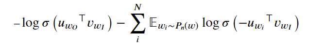
这个损失函数有点复杂,𝑢𝑤𝑂⊤ 是“输出”目标字词的嵌入向量(转置后的向量,即 ⊤ 符号的含义),𝑣𝑤𝐼是“输入”字词的嵌入向量。第一项的含义是
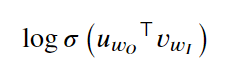
对输出词向量和输入词向量的内积运行 log-sigmoid 函数。对于第二项,先看看
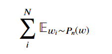
意思是对从噪点分布 𝑤𝑖∼𝑃𝑛(𝑤)中抽取的字词 𝑤𝑖求和。噪点分布是指不在输入字词的上下文中的词汇表。实际上,我们可以从词汇表里随机抽取字词来获得这些噪点字词。𝑃𝑛(𝑤)是一个任意概率分布,因此我们可以决定如何对抽取的字词设定权重。它可以是一个均匀分布,即抽取所有字词的概率是相同的。也可以根据每个字词出现在文本语料库(一元分布 𝑈(𝑤)里的频率进行抽样。论文作者根据实践发现,最佳分布是 𝑈(𝑤)3/4。
最后,在以下部分
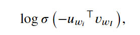
我们将对噪点向量与输入向量的内积否定结果运行 log-sigmoid 函数。
import torch from torch import nn import torch.optim as optim class SkipGramNeg(nn.Module): def __init__(self, n_vocab, n_embed, noise_dist=None): super().__init__() self.n_vocab = n_vocab self.n_embed = n_embed self.noise_dist = noise_dist # define embedding layers for input and output words self.in_embed = nn.Embedding(n_vocab,n_embed) self.out_embed = nn.Embedding(n_vocab,n_embed) # Initialize both embedding tables with uniform distribution def forward_input(self, input_words): # return input vector embeddings input_vectors = self.in_embed(input_words) return input_vectors def forward_output(self, output_words): # return output vector embeddings output_vectors = self.out_embed(output_words) return output_vectors def forward_noise(self, batch_size, n_samples): """ Generate noise vectors with shape (batch_size, n_samples, n_embed)""" if self.noise_dist is None: # Sample words uniformly noise_dist = torch.ones(self.n_vocab) else: noise_dist = self.noise_dist # Sample words from our noise distribution noise_words = torch.multinomial(noise_dist, batch_size * n_samples, replacement=True) device = "cuda" if model.out_embed.weight.is_cuda else "cpu" noise_words = noise_words.to(device) ## TODO: get the noise embeddings # reshape the embeddings so that they have dims (batch_size, n_samples, n_embed) noise_vectors = self.out_embed(noise_words).view(batch_size,n_sample,self.n_embed) return noise_vectors class NegativeSamplingLoss(nn.Module): def __init__(self): super().__init__() def forward(self, input_vectors, output_vectors, noise_vectors): batch_size, embed_size = input_vectors.shape # Input vectors should be a batch of column vectors input_vectors = input_vectors.view(batch_size, embed_size, 1) # Output vectors should be a batch of row vectors output_vectors = output_vectors.view(batch_size, 1, embed_size) # bmm = batch matrix multiplication # correct log-sigmoid loss out_loss = torch.bmm(output_vectors, input_vectors).sigmoid().log() out_loss = out_loss.squeeze() # incorrect log-sigmoid loss noise_loss = torch.bmm(noise_vectors.neg(), input_vectors).sigmoid().log() noise_loss = noise_loss.squeeze().sum(1) # sum the losses over the sample of noise vectors # negate and sum correct and noisy log-sigmoid losses # return average batch loss return -(out_loss + noise_loss).mean() 训练
下面是训练循环,如果有 GPU 设备的话,建议在 GPU 设备上训练模型。
device = 'cuda' if torch.cuda.is_available() else 'cpu' # Get our noise distribution # Using word frequencies calculated earlier in the notebook word_freqs = np.array(sorted(freqs.values(), reverse=True)) unigram_dist = word_freqs/word_freqs.sum() noise_dist = torch.from_numpy(unigram_dist**(0.75)/np.sum(unigram_dist**(0.75))) # instantiating the model embedding_dim = 300 model = SkipGramNeg(len(vocab_to_int), embedding_dim, noise_dist=noise_dist).to(device) # using the loss that we defined criterion = NegativeSamplingLoss() optimizer = optim.Adam(model.parameters(), lr=0.003) print_every = 1500 steps = 0 epochs = 5 # train for some number of epochs for e in range(epochs): # get our input, target batches for input_words, target_words in get_batches(train_words, 512): steps += 1 inputs, targets = torch.LongTensor(input_words), torch.LongTensor(target_words) inputs, targets = inputs.to(device), targets.to(device) # input, outpt, and noise vectors input_vectors = model.forward_input(inputs) output_vectors = model.forward_output(targets) noise_vectors = model.forward_noise(inputs.shape[0], 5) # negative sampling loss loss = criterion(input_vectors, output_vectors, noise_vectors) optimizer.zero_grad() loss.backward() optimizer.step() # loss stats if steps % print_every == 0: print("Epoch: {}/{}".format(e+1, epochs)) print("Loss: ", loss.item()) # avg batch loss at this point in training valid_examples, valid_similarities = cosine_similarity(model.in_embed, device=device) _, closest_idxs = valid_similarities.topk(6) valid_examples, closest_idxs = valid_examples.to('cpu'), closest_idxs.to('cpu') for ii, valid_idx in enumerate(valid_examples): closest_words = [int_to_vocab[idx.item()] for idx in closest_idxs[ii]][1:] print(int_to_vocab[valid_idx.item()] + " | " + ', '.join(closest_words)) print("...\n") 可视化字词向量
下面我们将使用 T-SNE 可视化高维字词向量聚类。T-SNE 可以将这些向量投射到二维空间里,同时保留局部结构。
%matplotlib inline %config InlineBackend.figure_format = 'retina' import matplotlib.pyplot as plt from sklearn.manifold import TSNE # getting embeddings from the embedding layer of our model, by name embeddings = model.in_embed.weight.to('cpu').data.numpy() viz_words = 380 tsne = TSNE() embed_tsne = tsne.fit_transform(embeddings[:viz_words, :]) fig, ax = plt.subplots(figsize=(16, 16)) for idx in range(viz_words): plt.scatter(*embed_tsne[idx, :], color='steelblue') plt.annotate(int_to_vocab[idx], (embed_tsne[idx, 0], embed_tsne[idx, 1]), alpha=0.7)
来源:https://blog.csdn.net/qq_36795658/article/details/98883513